Here’s a rewritten version of the blog post that’s more conversational, flows naturally, and keeps the original instructions intact while connecting better with the reader.
How to Make a Pie Chart in Google Sheets (2026)
By Deepti Pathak
February 22, 2026
Let’s be honest—data can feel overwhelming. But when you turn a few numbers into a clean, colorful pie chart? Suddenly, everything clicks. Whether you’re putting together a report, prepping for a meeting, or just trying to make sense of your own numbers, pie charts are one of the easiest ways to show how parts add up to a whole.
Google Sheets makes this surprisingly simple. No complicated tools, no steep learning curve. Here’s how to create a pie chart in just a few clicks.
How to Make a Pie Chart in Google Sheets
If you’ve never made one before, don’t worry—it’s almost embarrassingly easy. Here’s the step-by-step:
- Open Google Sheets and enter your data in a simple table.
- Select the columns and rows you want to include in your chart.
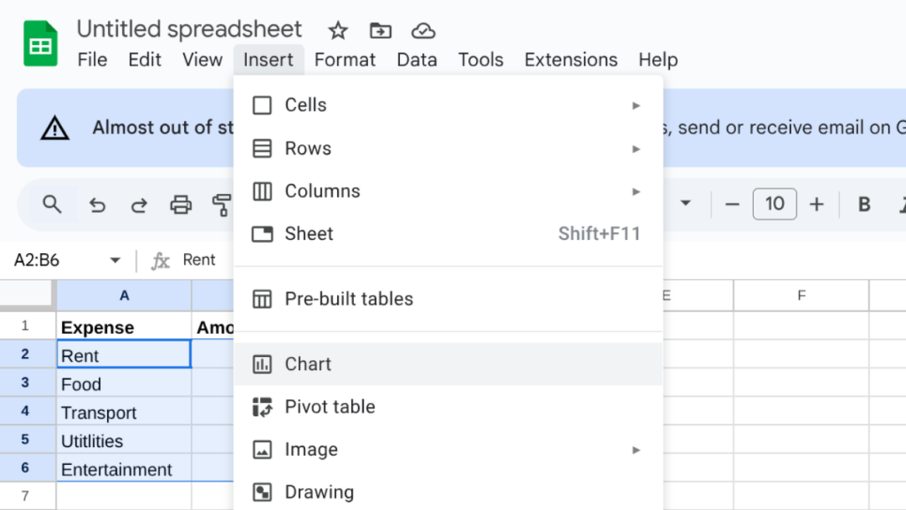
- Click Insert in the top menu, then choose Chart from the dropdown.
- Google Sheets might suggest a different chart type at first. That’s fine—just head over to the Chart Editor on the right and switch the chart type to Pie chart.
Once you’ve done that, the fun part begins. You can tweak the design, adjust the colors, and add your own personal touch to make the chart truly yours.
How to Make a 3D Pie Chart in Google Sheets
Want a little more visual flair? Turning your standard pie chart into a 3D version only takes a moment.
Once your chart is ready, follow these steps:
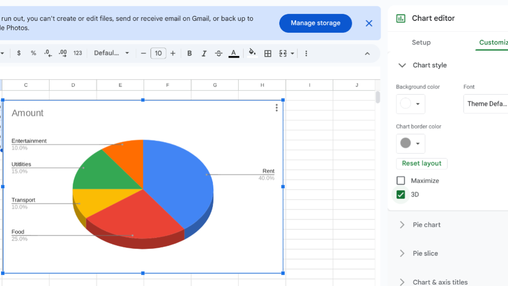
- Open the Chart Editor on the right.
- Click the Customize tab.
- Under Chart style, check the 3D box.
That’s it. Now you’ve got a chart with a bit more depth—great for presentations or when you want your data to stand out.
How to Show Percentages in Your Pie Chart
Sometimes a pie chart alone isn’t enough—you need the numbers to speak for themselves. Adding percentages helps people quickly understand the story behind the data.
Here’s how to make that happen:
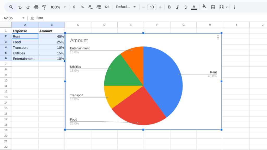
- Click on your pie chart to open the Chart Editor.
- Go to the Customize tab and expand the Pie chart section.
- Under Slice label, select Percentage from the dropdown.
Now, percentages will appear right on the slices. No more guessing—everyone can see the exact breakdown at a glance.
If you’d still like a legend to help identify each slice, here’s how to add it:
- Under Customize, open the Legend section.
- Choose where you want the legend to appear—top, bottom, left, or right.
Now your chart shows both percentages inside the slices and a clear legend to match each value to its category. Clean, professional, and easy to read.
Wrapping It Up
Whether you’re building a business report, working on a school project, or just trying to organize your personal budget, a well-made pie chart can turn raw numbers into a story that makes sense.
Google Sheets gives you all the tools you need—without the complexity. With a few clicks, you can add color, percentages, even a 3D effect, and present your data in a way that feels both polished and approachable.
So next time you’re staring at a spreadsheet, give it a try. You might be surprised how satisfying it is to watch your data come full circle.